2.3 Descriptive and Inferential Statistics
Learning Objectives
- Describe descriptive statistics and know how to produce them.
- Describe inferential statistics and why they are used.
Descriptive statistics
In the previous section, we looked at some of the research designs psychologists use. In this section, we will provide an overview of some of the statistical approaches researchers take to understanding the results that are obtained in research. Descriptive statistics are the first step in understanding how to interpret the data you have collected. They are called descriptive because they organize and summarize some important properties of the data set. Keep in mind that researchers are often collecting data from hundreds of participants; descriptive statistics allow them to make some basic interpretations about the results without having to eyeball each result individually.
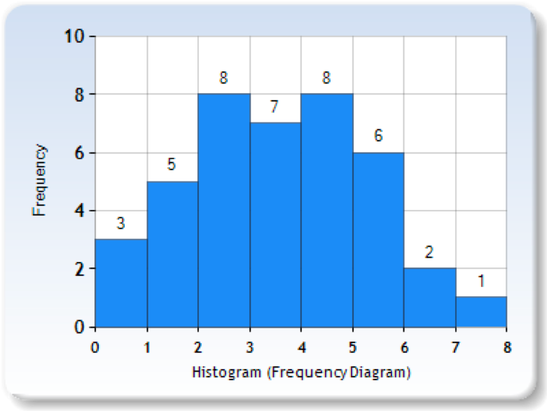
Let’s work through a hypothetical example to show how descriptive statistics help researchers to understand their data. Let’s assume that we have asked 40 people to report how many hours of moderate-to-vigorous physical activity they get each week. Let’s begin by constructing a frequency distribution of our hypothetical data that will show quickly and graphically what scores we have obtained.
| Number of People | Hours of Exercise |
| 1 | 7 |
| 2 | 6 |
| 6 | 5 |
| 8 | 4 |
| 7 | 3 |
| 8 | 2 |
| 5 | 1 |
| 3 | 0 |
We can now construct a histogram that will show the same thing on a graph (see Figure 2.5). Note how easy it is to see the shape of the frequency distribution of scores.
Many variables that psychologists are interested in have distributions where most of the scores are located near the centre of the distribution, the distribution is symmetrical, and it is bell-shaped (see Figure 2.6). A data distribution that is shaped like a bell is known as a normal distribution. Normal distributions are common in human traits because of the tendency for variability; traits like intelligence, wealth, shoe size, and so on, are distributed such that relatively few people are either extremely high or low scorers, and most people fall somewhere near the middle.

A distribution can be described in terms of its central tendency — that is, the point in the distribution around which the data are centred — and its dispersion or spread. The arithmetic average, or arithmetic mean, symbolized by the letter M, is the most commonly used measure of central tendency. It is computed by calculating the sum of all the scores of the variable and dividing this sum by the number of participants in the distribution, denoted by the letter N. In the data presented in Figure 2.6, the mean height of the students is 67.12 inches (170.48 cm). The sample mean is usually indicated by the letter M.
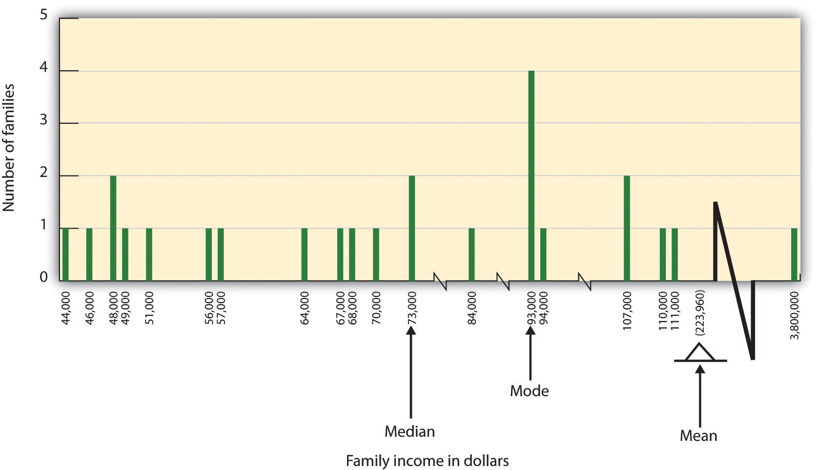
In some cases, however, the data distribution is not symmetrical. This occurs when there are one or more extreme scores, known as outliers, at one end of the distribution. Consider, for instance, the variable of family income (see Figure 2.7), which includes an outlier at a value of $3,800,000. In this case, the mean is not a good measure of central tendency. Although it appears from Figure 2.7 that the central tendency of the family income variable should be around $70,000, the mean family income is actually $223,960. The single very extreme income has a disproportionate impact on the mean, resulting in a value that does not well represent the central tendency.
The median is used as an alternative measure of central tendency when distributions are not symmetrical. The median is the score in the centre of the distribution, meaning that 50% of the scores are greater than the median and 50% of the scores are less than the median. In our case, the median household income of $73,000 is a much better indication of central tendency than is the mean household income of $223,960.
A final measure of central tendency, known as the mode, represents the value that occurs most frequently in the distribution. You can see from Figure 2.7 that the mode for the family income variable is $93,000; it occurs four times.
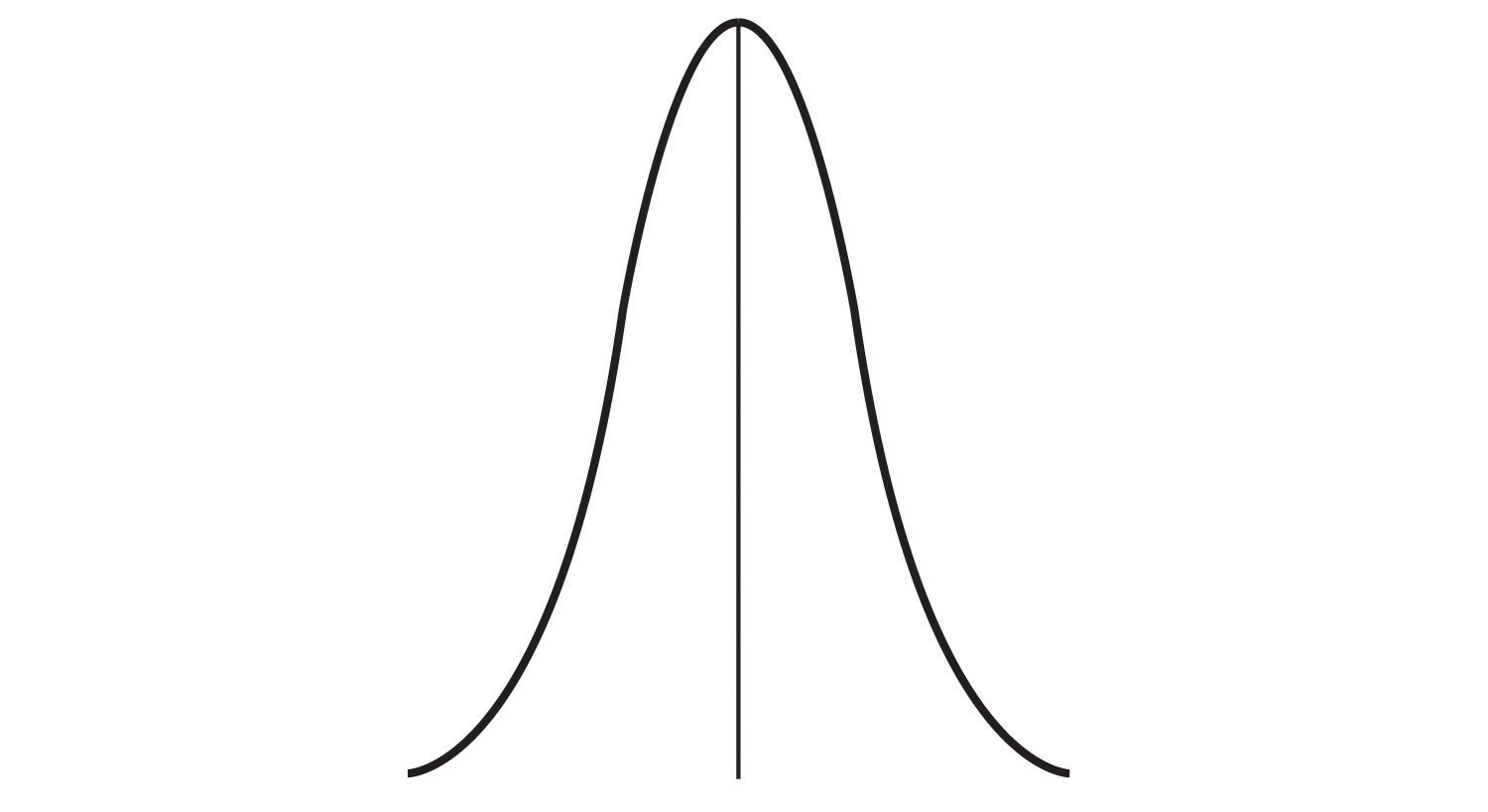
In addition to summarizing the central tendency of a distribution, descriptive statistics convey information about how the scores of the variable are spread around the central tendency. Dispersion refers to the extent to which the scores are all tightly clustered around the central tendency (see Figure 2.8). Here, there are many scores close to the middle of the distribution.
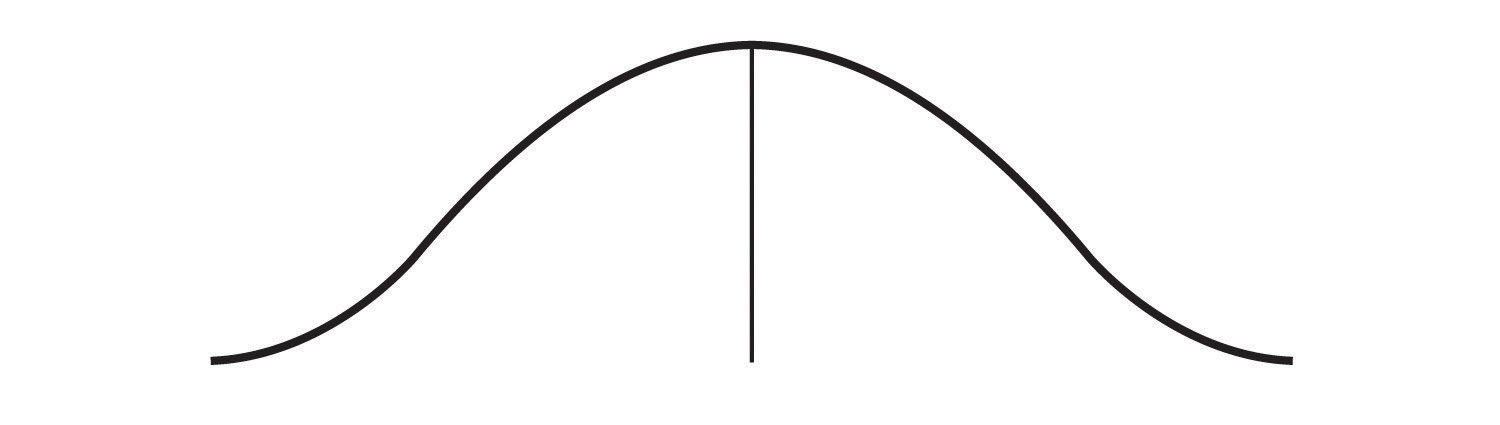
In other instances, they may be more spread out away from it (see Figure 2.9). Here, the scores are further away from the middle of the distribution.
One simple measure of dispersion is to find the largest (i.e., the maximum) and the smallest (i.e., the minimum) observed values of the variable and to compute the range of the variable as the maximum observed score minus the minimum observed score. You can check that the range of the height variable shown in Figure 2.6 above is 72 – 62 = 10.
The standard deviation, symbolized as s, is the most commonly used measure of variability around the mean. Distributions with a larger standard deviation have more spread. Those with small deviations have scores that do not stray very far from the average score. Thus, standard deviation is a good measure of the average deviation from the mean in a set of scores. In the examples above, the standard deviation of height is s = 2.74, and the standard deviation of family income is s = $745,337. These standard deviations would be more informative if we had others to compare them to. For example, suppose we obtained a different sample of adult heights and compared it to those shown in Figure 2.6 above. If the standard deviation was very different, that would tell us something important about the variability in the second sample as compared to the first. A more relatable example might be student grades: a professor could keep track of student grades over many semesters. If the standard deviations were relatively similar from semester to semester, this would indicate that the amount of variability in student performance is fairly constant. If the standard deviation suddenly went up, that would indicate that there are more students with very low scores, very high scores, or both. It’s useful to see how standard deviation is calculated: a good demonstration can be found at Khan Academy.
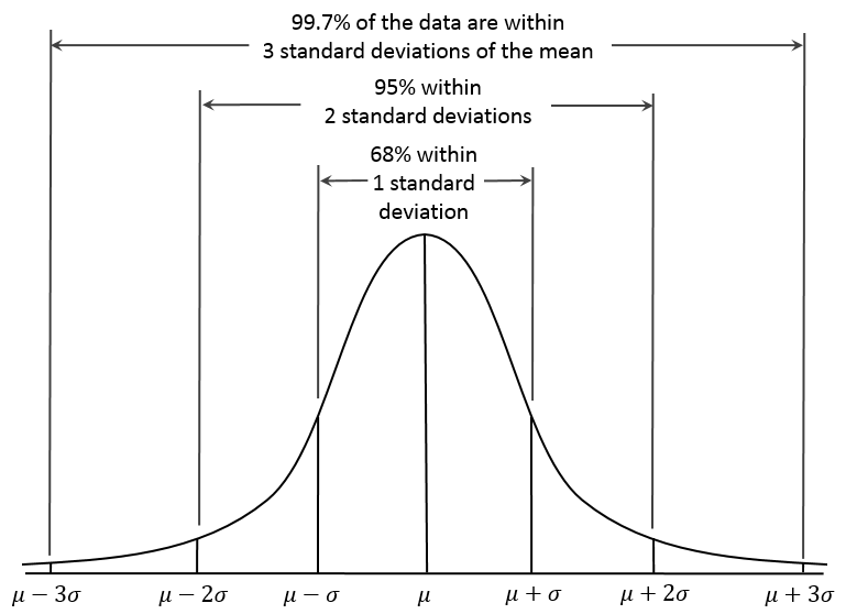
The standard deviation in the normal distribution has some interesting properties (see Figure 2.10). Approximately 68% of the data fall within 1 standard deviation above or below the mean score: 34% fall above the mean, and 34% fall below. In other words, about 2/3 of the population are within 1 standard deviation of the mean. Therefore, if some variable is normally distributed (e.g., height, IQ, etc.), you can quickly work out where approximately 2/3 of the population fall by knowing the mean and standard deviation.
Inferential statistics
We have seen that descriptive statistics are useful in providing an initial way to describe, summarize, and interpret a set of data. They are limited in usefulness because they tell us nothing about how meaningful the data are. The second step in analyzing data requires inferential statistics. Inferential statistics provide researchers with the tools to make inferences about the meaning of the results. Specifically, they allow researchers to generalize from the sample they used in their research to the greater population, which the sample represents. Keep in mind that psychologists, like other scientists, rely on relatively small samples to try to understand populations.
This is not a textbook about statistics, so we will limit the discussion of inferential statistics. However, all students of psychology should become familiar with one very important inferential statistic: the significance test. In the simplest, non-mathematical terms, the significance test is the researcher’s estimate of how likely it is that their results were simply the result of chance. Significance testing is not the same thing as estimating how meaningful or large the results are. For example, you might find a very small difference between two experimental conditions that is statistically significant.
Typically, most researchers use the convention that if significance testing shows that a result has a less than 5% probability of being due to chance alone, the result is considered to be real and to generalize to the population. If the significance test shows that the probability of chance causing the outcome is greater than 5%, it is considered to be a non-significant result and, consequently, of little value; non-significant results are more likely to be chance findings and, therefore, should not be generalized to the population. Significance tests are reported as p values, for example, p< .05 means the probability of being caused by chance is less than 5%. P values are reported by all statistical programs so students no longer need to calculate them by hand. Most often, p values are used to determine whether or not effects detected in the research are present. So, if p< .05, then we can conclude that an effect is present, and the difference between the two groups is real.
Thus, p values provide information about the presence of an effect. However, for information about how meaningful or large an effect is, significance tests are of little value. For that, we need some measure of effect size. Effect size is a measure of magnitude; for example, if there is a difference between two experimental groups, how large is the difference? There are a few different statistics for calculating effect sizes.
In summary, statistics are an important tool in helping researchers understand the data that they have collected. Once the statistics have been calculated, the researchers interpret their results. Thus, while statistics are heavily used in the analysis of data, the interpretation of the results requires a researcher’s knowledge, analysis, and expertise.
Key Takeaways
- Descriptive statistics organize and summarize some important properties of the data set. Frequency distributions and histograms are effective tools for visualizing the data set. Measures of central tendency and dispersion are descriptive statistics.
- Many human characteristics are normally distributed.
- Measures of central tendency describe the central point around which the scores are distributed. There are three different measures of central tendency.
- The range and standard deviation show the dispersion of scores as well as the shape of the distribution of the scores. The standard deviation of the normal distribution has some special properties.
- Inferential statistics provide researchers with the tools to make inferences about the meaning of the results, specifically about generalizing from the sample they used in their research to the greater population, which the sample represents.
- Significance tests are commonly used to assess the probability that observed results were due to chance. Effect sizes are commonly used to estimate how large an effect has been obtained.
Exercises and Critical Thinking
- Keep track of something you do over a week, such as your daily amount of exercise, sleep, cups of coffee, or social media time. Record your scores for each day. At the end of the week, construct a frequency distribution of your results, and draw a histogram that represents them. Calculate all three measures of central tendency, and decide which one best represents your data and why. Invite a friend or family member to participate, and do the same for their data. Compare your data sets. Whose shows the greatest dispersion around the mean, and how do you know?
- The data for one person cannot generalize to the population. Consider why people might have different scores than yours.
Image Attribution
Figure 2.5. Used under a CC BY-NC-SA 4.0 license.
Figure 2.6. Used under a CC BY-NC-SA 4.0 license.
Figure 2.7. Used under a CC BY-NC-SA 4.0 license.
Figure 2.8. Used under a CC BY-NC-SA 4.0 license.
Figure 2.9. Used under a CC BY-NC-SA 4.0 license.
Figure 2.10. Empirical Rule by Dan Kernler is used under a CC BY-SA 4.0 license.
Long Descriptions
Figure 2.7. Of the 25 families, 24 families have an income between $44,000 and $111,000, and only one family has an income of $3,800,000. The mean income is $223,960, while the median income is $73,000.
